[display-name-category]

[post_author]

In my previous article posts, I spoke about different implementations that can be carried out with Excel in order to better analyze data and help you when you are optimizing your campaigns.

On this occasion, I will give you some pointers on how to use Excel if you need to come up with some reports for your own purposes or even if you need to deliver them to a Client or to upper management within your company.

First off, you need to assure you have the correct date range set within your campaign. This should be in accordance to what you want to report. To best exemplify my point in this article, I will use a “Last Month” date range.

There are different aspects of the account that can be taken in consideration for reporting purposes. I will begin this article by mentioning how to gather data at a campaign level. Please make sure that you have “All Online Campaigns” selected in the account and then select “Download Report”:

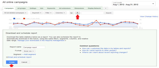
Open the file that has been downloaded in Excel. The first thing I recommend you to do within this file is to erase any rows mentioning totals, as these may skew the data when we try to create a report. Furthermore, do the same with any columns that may not be relevant to the data that you want.

Now you will need to select all the data from the columns in question; all the way through the last row of data. After you have done this, you need to insert a pivot table. Just like this:

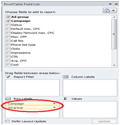
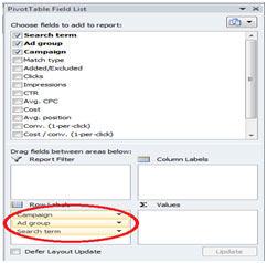
This action will insert a pivot table with the data selected in a new sheet by default for you. You now need to select the right data that you will be displaying in your pivot table. You do this by dragging the elements respectively in the “PivotTable Field List”. At campaign level, I use the following layout:

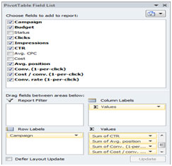
The next thing to do will be to change the way the stats are shown. The following values could be left as they are:

• Budget

• Clicks

• Impressions

• Avg. Position

• Conv. (1-per-click)

• Cost / Conv. (1-per-click)

But the following values should be modified:

• CTR

• Conv. Rate (1-per-click)

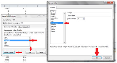
The way you modify them is by clicking on the arrow next to their name in the “Values” section of the “Field List”, as so:

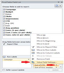
Within the window pop up, you can change this value to reflect an “Average” and display it via the “Percentage” option, just like this:

We are almost done with our report.

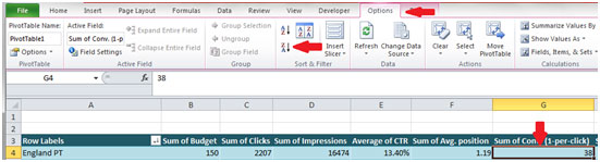
The following step will be to make your pivot table look more attractive and concise. First, I will recommend you to sort your data depending on the metric that is most important for you. To do this, you only need to select the first cell of data in the column that you deem most important and then sort from higher to lower amount. Such as this:

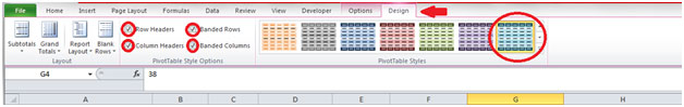
This will allow you to display the stats based on your most important metric. Last but not least, we need to add some colors in your table.

Select a design that best suits your needs and make sure you have all the values properly separated. As so:

This should leave you with a thorough table that will cover all the metrics for the previous month’s performance. Since it will have all the necessary information and will look nice and well-sorted, you can just send it over in an email with a little explanation to anyone interested in reviewing the information further.

You can perform this same set up for different levels of your campaign; it will actually allow you to report information in the same manner within the following levels:

• Ad Group

• Keyword

• Search Term

The only difference will be that when adding the values that you want to use in your pivot table, you will need to add the respective level to the “Row Labels”. So your set up for the pivot tables should look like this:

• Ad Groups:

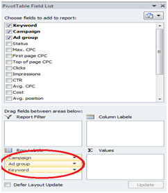
• Keywords:

• Search Terms:

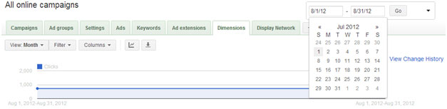
Now, last but not least, I will like to also explain how to run a quick report to compare the performance over two months by using the “Dimensions” tab.

First of all, you will need to make sure you have selected the last two complete months within the date range. You can start by selecting “Last Month”, as we did in our previous examples. Then,  perform a “Custom Date” and select the first day of the previous month for the one already selected. Such as this:

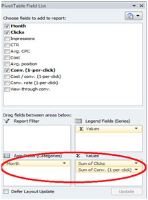
Now you will do just as we previously had done with the other files. You need to delete any rows showing totals, other columns and rows that you don’t need and insert a pivot table. For the set-up of this pivot table, I will recommend you use only a couple of metrics as values. This is because we will create a graph to better visualize this last report. If you add too many values however, the graph can appear odd, so be forewarned.

You can set-up your pivot table like this:

Now that you have this prepared, you will just need to insert a pivot graph to reflect the date you have within your table. Just like this:

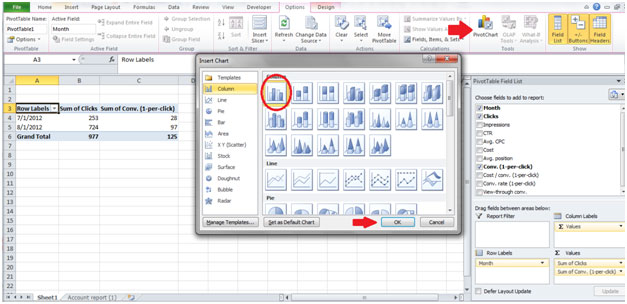
I used a default 2-D column design, but feel free to use any other one you think will best reflect your data. Finally, and as we previously attempted, you can give the pivot table a different design, set of colors and divvy it up with different metrics.

By implementing these quick tips, you can easily come up with some tables and even graphs to report your performance to your superiors, clients, blogs, or anything that you need. Feel free to play with them and try different settings and designs to see if you can make them look better and even more professional.